I found a blog in the web at which uses Euler to analyze sound, implementing a very simple code to scale up the rate of a sound sample.
For a demonstration, I generate a sound with harmonics using a sample rate of 8820Hz.
>r=8820; ...
 t=soundsec(2,rate=r); ...
 s=sin(t*440)+sin(2t*440)/2+sin(3t*440)/3;
The time ticks t[i] can be generated with soundsec, and the sound with the matrix language. The sound can be analized very easily using FFT in Euler.
>analyzesound(s,rate=r):
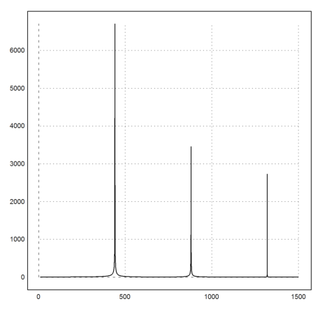
We can clearly see and hear the frequencies.
>playwave(s,rate=r);
We want to increase the sample rate of 8820Hz to 22050Hz. Obviously, this requires some interpolation.
First, we use a very simple scheme. Effectively, we repeat the sound items as many times as is necessary.
>i=round(linspace(1,cols(t),cols(t)*2.75-1),0);
This index vector contains the indices to take the from the original sample.
>i[1:10], i[-10:-1]
[1,  1,  2,  2,  2,  3,  3,  4,  4,  4]
[17637,  17637,  17637,  17638,  17638,  17639,  17639,  17639,  17640,
17640]
>s1=s[i]; r1=r*2.75;
The original sound is smooth.
>plot2d(s[1:100]):
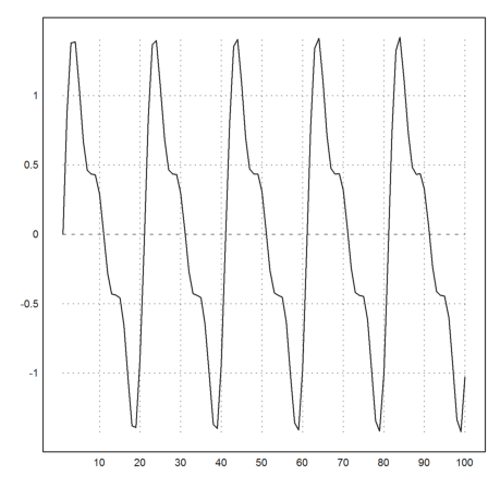
The interpolated sound contains lots of steps.
>plot2d(s1[1:275]):
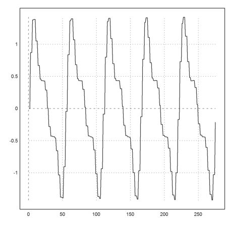
The analysis looks good, however.
>analyzesound(s1,rate=r1):
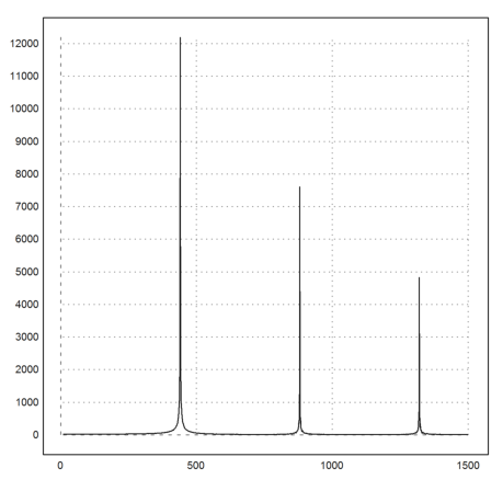
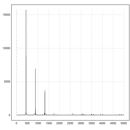
But there are many higher frequencies, which are artifacts generated by the steps.
>analyzesound(s1,rate=r1,fmax=5000):

And in fact, you can hear those artifacts. The sound sounds terrible.
>playwave(s1,rate=r1);
The blog at the address above uses a different, more complicated scheme.
>function scaleup (s) ...
 n=1;
 idx=0;
 res=zeros(1,cols(s)*2.5);
 for i=1 to cols(res)
   idx=idx+93;
   if idx>256 then idx=idx-256; n=n+1; endif;
   res[i]=s[n];
 end;
 return res
 endfunction
>s2=scaleup(s);
The result has even more high frequencies.
>analyzesound(s2,rate=r1,fmax=5000):
And it sounds even worse.
>playwave(s2,rate=r1);
Of course, we need to interpolate the data much better.
In the following, I use a linear interpolation between adjacent data points. E.g., I set
![]()
where delta is the time scale of the original sound.
In Euler, this can be done in the following way. First, we need the indices we would like to take, evenly spaced along the indices of our sound.
>i=linspace(1,cols(t),cols(t)*2.75-1); i[1:20]
[1,  1.36362,  1.72725,  2.09087,  2.45449,  2.81812,  3.18174,
3.54536,  3.90899,  4.27261,  4.63623,  4.99986,  5.36348,  5.7271,
6.09073,  6.45435,  6.81797,  7.1816,  7.54522,  7.90884]
Then we compute integer indices and the weights.
>i1=floor(i); f1=1-(i-i1);
>i2=ceil(i); f2=1-(i2-i);
Finally, we can assemble the new sound.
>s3=f1*s[i1]+f2*s[i2];
It looks very clean now.
>analyzesound(s3,rate=r1,fmax=5000):
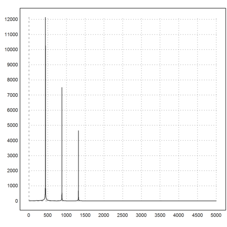
And it sound very clean.
>playwave(s3,rate=r1);